Utils

as_percentage

 as_percentage (x, ndigits=2)

source

cut_model_by_name

 cut_model_by_name (model, cut)

classifier = resnet34()
body = cut_model_by_name(classifier, 'avgpool')
test(body, 'avgpool', hasattr)
assert not hasattr(body, 'fc')

source

MLP

 MLP (logits:Optional[int], hidden_depth=5, hidden_width=512,
      features_dim=None)

A Multilayer Perceptron comprized of linear layers with ReLU activations.

	Type	Default	Details
logits	typing.Optional[int]		Number of logits. pass `None` to not include a logits layer after the hidden layers
hidden_depth	int	5	Number of hidden layers
hidden_width	int	512	Number of neurons in each hidden layer
features_dim	NoneType	None	Number of neurons in the last hidden layer. Pass `None` to use the same value as the other hidden layers

source

Threshold

 Threshold ()

Classifies 1D inputs into 2 classes, based on whether they surpass a threshold or not

threshold = Threshold()
with torch.no_grad():
    threshold.t[0] = 3

test_eq(threshold(torch.arange(10)).argmax(1), torch.tensor([1]*3+[0]*7))

Since this is such a simple model, we can fit it to data without iterative optimization:

source

Threshold.fit

 Threshold.fit (x, y)

Picks a threshold that maximizes the empirical accuracy

threshold = Threshold()
x = torch.randint(high=10, size=(100,))
chosen_threshold, _ = threshold.fit(x, x < 3)

test_close(chosen_threshold, 3, eps=1)

Experiments

Sometimes we want to test a certain procedure (e.g. training a model) multiple times, examine the distribution of the resulting stats. For example, we might want to train and test the same model on different train-test splits, or even the same split to examine the effect of training stochasticity on the results.

While tools like TensorBoard can be used for an in-depth analysis of the whole process (e.g. loss-by-epoch graphs), sometimes we just want to note the distribution of the end results.

Averaging over multiple runs also gives more stable results, for example cross-validation gives a more accurate estimate to the model’s performance than training once.

source

RepeatedExperiment

 RepeatedExperiment (model:torch.nn.modules.module.Module,
                     data:List[fastai.data.core.Datasets], seed:int=0)

Runs multiple independent iterations of the same procedure, and combines the results

	Type	Default	Details
model	Module		The model to be used in each iteration. Parameter are reset to their initial values before each iteration
data	typing.List[fastai.data.core.Datasets]		A list of `Datasets`, each representing a different iteration. A `Dataloaders` of the current `Datasets` is available via `self.dls`
seed	int	0	Used for reproducibility of results. Use `None` to avoid reproducibility

source

ExperimentalResults

 ExperimentalResults (stats:List[Any])

Provides various ways of examining the results of a RepeatedExperiment

source

RepeatedExperiment.run

 RepeatedExperiment.run ()

Runs the experiment, returning the results as an ExperimentalResults

For example, we can train a linear classifier for MNIST multiple times and check distribution of accuracies:

class LinearMNIST(RepeatedExperiment):
    def iteration(self):
        learn = Learner(self.dls, self.model, metrics=accuracy)
        learn.fit(1)
        return dict(zip(['loss', 'accuracy'], learn.validate()))
    
res = LinearMNIST(model=nn.Sequential(nn.Flatten(), nn.Linear(28*28, 2)),
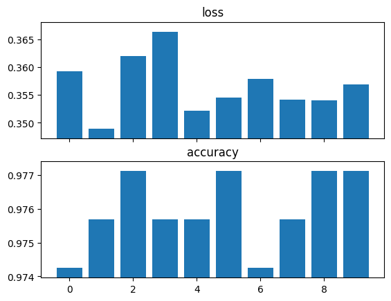
                  data=[TinyMNIST() for _ in range(10)]).run()

res.stats

[{'loss': 0.3591866195201874, 'accuracy': 0.9742489457130432},
 {'loss': 0.34896886348724365, 'accuracy': 0.9756795167922974},
 {'loss': 0.3619726896286011, 'accuracy': 0.9771101474761963},
 {'loss': 0.3663684129714966, 'accuracy': 0.9756795167922974},
 {'loss': 0.35216033458709717, 'accuracy': 0.9756795167922974},
 {'loss': 0.35451024770736694, 'accuracy': 0.9771101474761963},
 {'loss': 0.35790905356407166, 'accuracy': 0.9742489457130432},
 {'loss': 0.3541954755783081, 'accuracy': 0.9756795167922974},
 {'loss': 0.3539672791957855, 'accuracy': 0.9771101474761963},
 {'loss': 0.3568763732910156, 'accuracy': 0.9771101474761963}]

source

ExperimentalResults.collated_stats

 ExperimentalResults.collated_stats ()

res.collated_stats

{'loss': array([0.35918662, 0.34896886, 0.36197269, 0.36636841, 0.35216033,
        0.35451025, 0.35790905, 0.35419548, 0.35396728, 0.35687637]),
 'accuracy': array([0.97424895, 0.97567952, 0.97711015, 0.97567952, 0.97567952,
        0.97711015, 0.97424895, 0.97567952, 0.97711015, 0.97711015])}

source

ExperimentalResults.plot_stats

 ExperimentalResults.plot_stats ()

res.plot_stats()

source

ExperimentalResults.stat_means

 ExperimentalResults.stat_means ()

res.stat_means

{'loss': 0.35661153495311737, 'accuracy': 0.9759656548500061}

source

ExperimentalResults.stat_stds

 ExperimentalResults.stat_stds ()

res.stat_stds

{'loss': 0.004772754486396994, 'accuracy': 0.0010705668573123257}