Plotting Feature Space

Visualizing low-dimensional feature spaces

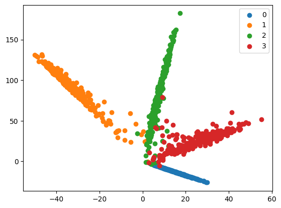
Since the backbone (in charge of embedding in feature space) plays such an intergral role in similarity learning, it’s natural that we’d want to examine it. While it’s usually too high-dimensional to plot directly, we could force it to be low-dimensional for the purpose of plotting.

---

source

plot_dataset_embedding

 plot_dataset_embedding (dataset:fastai.data.core.Datasets,
                         feature_extractor, num_samples_per_class=300,
                         normalize_features=False, *args, **kwargs)

In order to properly classify using only 3 features, we should pick a relatively simple dataset. Let’s use MNIST:

from torch import nn

from fastai_datasets.all import *

from similarity_learning.utils import *
from similarity_learning.siamese import *
from similarity_learning.pair_matching import *

mnist = MNIST()
mnist = mnist.by_target['0'] + mnist.by_target['1'] + mnist.by_target['2'] + mnist.by_target['3']

100.00% [10/10 00:00<00:00]

learn = Learner(mnist.dls(), MLP(10, features_dim=2), metrics=accuracy)
learn.fit(1)

epoch	train_loss	valid_loss	accuracy	time
0	0.097074	0.062883	0.982680	00:11

plot_dataset_embedding(mnist, cut_model_by_name(learn.model, 'hidden_layers'))

100.00% [4/4 00:00<00:00]

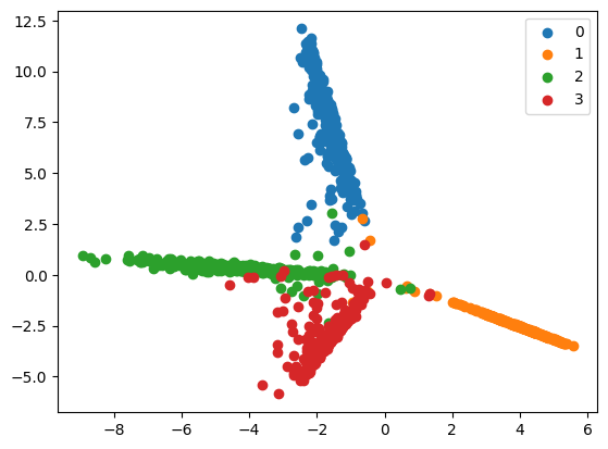
Compare with training a ThresholdSiamese and extracting the backbone:

learn = Learner(Pairs(mnist, 1).dls(), ThresholdSiamese(MLP(None, features_dim=2)), metrics=accuracy)
learn.fit(1)

epoch	train_loss	valid_loss	accuracy	time
0	0.314940	0.277123	0.966314	00:24

plot_dataset_embedding(mnist, learn.model.distance.backbone)

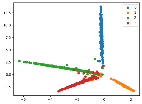
And with training a backbone with ContrastiveLoss

learn = Learner(Pairs(mnist, 1).dls(), DistanceSiamese(MLP(None, features_dim=2)), ContrastiveLoss())
learn.fit(1)

epoch	train_loss	valid_loss	time
0	0.048055	0.039739	00:25

plot_dataset_embedding(mnist, learn.model.backbone)